Inverse analysis of ASTM C1609
Inverse analysis · unnotched beam · strain-based
Back-calculate the tension stress-strain law of an FRC or UHPC matrix from the load-deflection curve of a four-point (ASTM C1609) or three-point bending test on an unnotched beam.
Inverse analysis. Patel, D., Pleesudjai, C., Bakhshi, M., Nasri, V., and Mobasher, B. (2025). Back-calculation of mechanical properties of fiber-reinforced concrete in tunnel lining segments. Structural Concrete, 26, 6019–6040. doi:10.1002/suco.70052
The software. Patel, D., Pleesudjai, C., and Mobasher, B. (2026). An interactive inverse-analysis and design tool for reinforced UHPC beams. Fourth International Interactive Symposium on Ultra-High Performance Concrete, paper 44.
What you need
- The beam dimensions, the span, the loading arrangement and the load spacing of the test.
- The compressive strength of the mix. A measured modulus helps but is not required.
- The load-deflection record of one specimen as a two-column file, deflection then load, in the units you will select in the module. See Test data files.
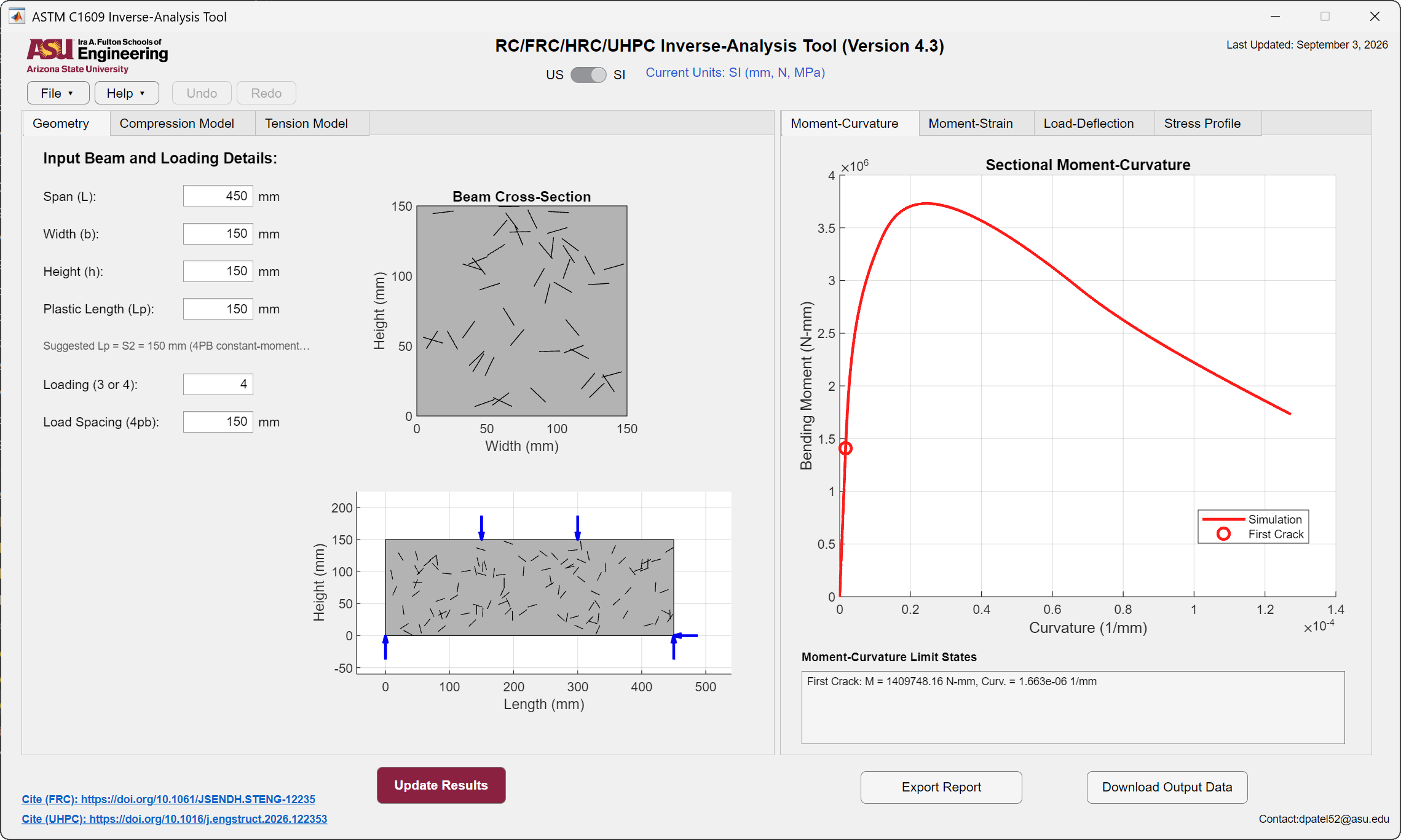
This project, and the module's own example
File → Open Example Project loads the reference project selected for this module, which may be a different specimen from the one pictured here, depending on the build. The steps below are written against the downloadable project above so that the screenshots match what you see. Either project exercises the module in the same way.
Step 1 · Geometry
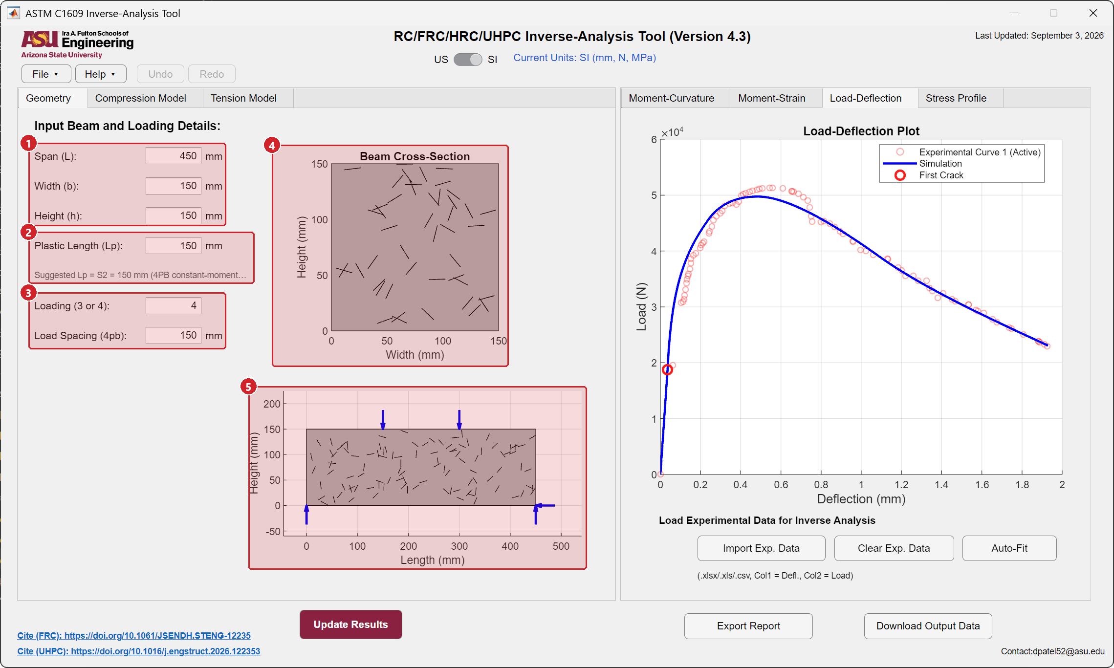
- Span, width and height. The clear span between the supports and the section dimensions. Set the unit system with the US / SI switch before typing.
- Plastic length. The zone over which the post-peak curvature localizes. The suggested value is printed under the box: the constant-moment zone \(S_2\) for four-point bending, the depth \(h\) for three-point bending. Keep the suggestion unless you have a reason to change it.
- Loading and load spacing. Type 4 for four-point bending (ASTM C1609, loads at the third points give \(S_2 = L/3\)) or 3 for three-point bending. The load spacing is used only in four-point bending.
- Cross-section drawing. A random fiber pattern on the section, drawn to scale.
- Beam elevation. Supports and loads at the positions you entered. Check that the arrows are where the machine put them.
| Input | Symbol | Unit | Example |
|---|---|---|---|
| Span (L) | \(L\) | mm | 450 |
| Width (b) | \(b\) | mm | 150 |
| Height (h) | \(h\) | mm | 150 |
| Plastic Length (Lp) | \(L_p\) | mm | 150 |
| Loading (3 or 4) | 4 | ||
| Load Spacing (4pb) | \(S_2\) | mm | 150 |
| Input | Symbol | Unit | Example |
|---|---|---|---|
| Span (L) | \(L\) | in | 18 |
| Width (b) | \(b\) | in | 6 |
| Height (h) | \(h\) | in | 6 |
| Plastic Length (Lp) | \(L_p\) | in | 6 |
| Loading (3 or 4) | 4 | ||
| Load Spacing (4pb) | \(S_2\) | in | 6 |
Step 2 · Compression model
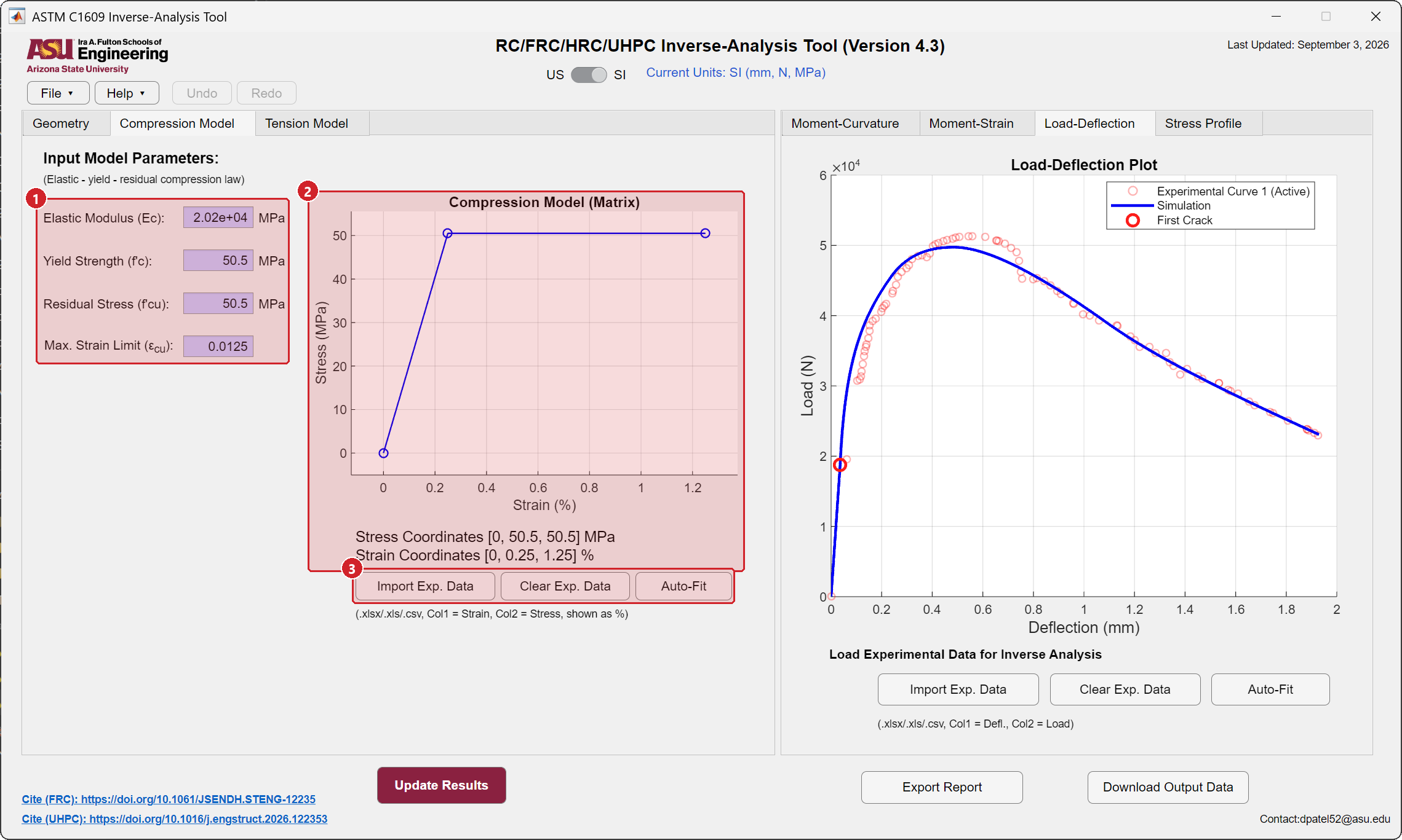
- Enter the compression law. Elastic modulus \(E_c\), compressive strength \(f'_c\), residual stress \(f'_{cu}\) after the peak, and the maximum strain \(\varepsilon_{cu}\). For an elastic-perfectly plastic law set \(f'_{cu} = f'_c\). The compressive strength also drives the suggested tension values on the next tab.
- Check the plot. The three coordinates are listed under the plot. Drag a vertex to adjust the law by eye.
- Import a measured curve if a cylinder test with strain readings exists, then press Auto-Fit on this tab to fit the compression law to it. Most users skip this step.
The compression law is held fixed during the tension Auto-Fit. In a flexural test of a strain-softening FRC the compression zone stays elastic, so the exact post-peak values matter little. In UHPC they matter, and a measured strength should be used.
Step 3 · Tension model
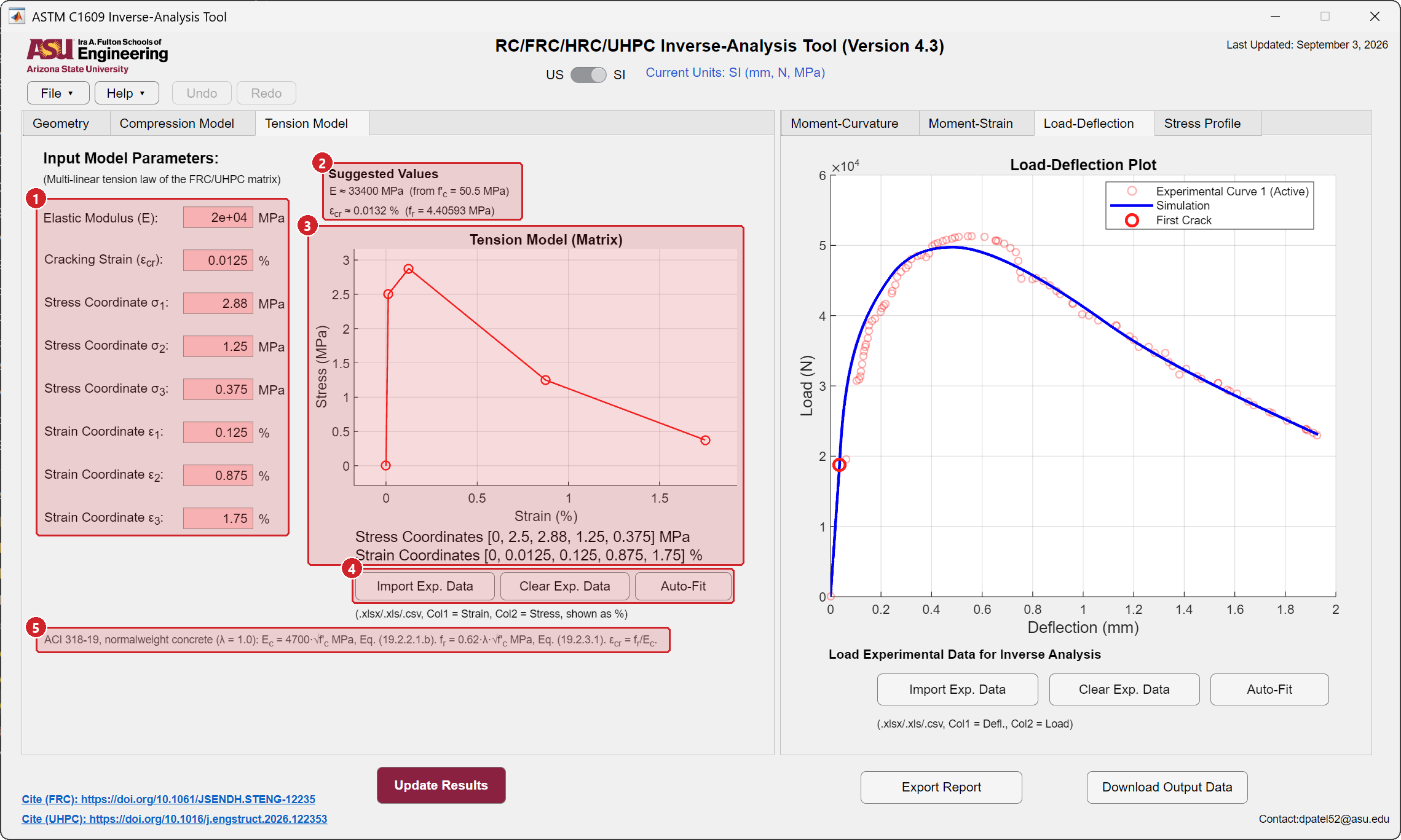
- Enter a starting law. Elastic modulus \(E\), cracking strain \(\varepsilon_{cr}\), then three stress coordinates \(\sigma_1, \sigma_2, \sigma_3\) and their strains \(\varepsilon_1, \varepsilon_2, \varepsilon_3\). Auto-Fit will replace all of them except \(E\), so a rough guess is enough. Keep the strains increasing.
- Suggested values. \(E\) and \(\varepsilon_{cr}\) computed from the compressive strength with the ACI 318-19 expressions. Copy them into the boxes when nothing better is known.
- The plot. The five coordinates are listed under it, starting at the origin and the cracking point. Drag any vertex to change the law and watch the result tabs follow.
- Import, clear, fit a direct tension test. Only when uniaxial tension data exist. The inverse analysis from the flexural test is done on the Load-Deflection tab, not here.
- The formulas behind the suggestions, printed for reference.
| Input | Symbol | Unit | Example |
|---|---|---|---|
| Elastic Modulus (E) | \(E\) | MPa | 20 000 |
| Cracking Strain | \(\varepsilon_{cr}\) | % | 0.0125 |
| Stress Coordinate 1, 2, 3 | \(\sigma_1, \sigma_2, \sigma_3\) | MPa | 2.88, 1.25, 0.375 |
| Strain Coordinate 1, 2, 3 | \(\varepsilon_1, \varepsilon_2, \varepsilon_3\) | % | 0.125, 0.875, 1.75 |
| Input | Symbol | Unit | Example |
|---|---|---|---|
| Elastic Modulus (E) | \(E\) | psi | 2 900 000 |
| Cracking Strain | \(\varepsilon_{cr}\) | % | 0.0125 |
| Stress Coordinate 1, 2, 3 | \(\sigma_1, \sigma_2, \sigma_3\) | psi | 417, 181, 54.4 |
| Strain Coordinate 1, 2, 3 | \(\varepsilon_1, \varepsilon_2, \varepsilon_3\) | % | 0.125, 0.875, 1.75 |
The cracking stress is \(\sigma_{cr} = E\,\varepsilon_{cr}\), 2.5 MPa in the example. A first coordinate above it, as in the example, describes a strain-hardening response after cracking; a first coordinate below it describes strain softening.
Step 4 · Import the test curve
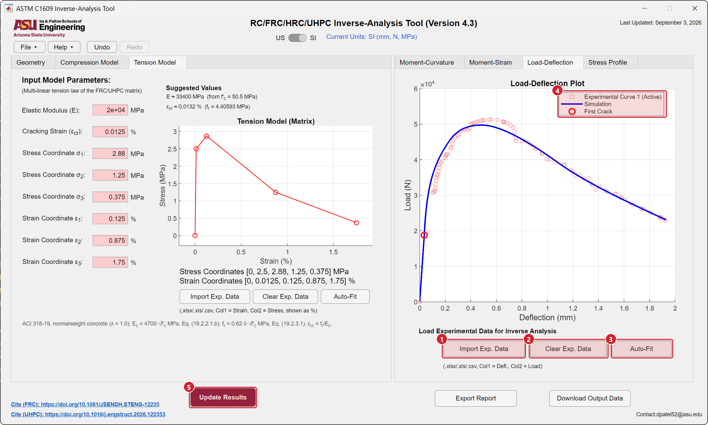
- Import Exp. Data. Choose the two-column file. The curve appears as open circles and becomes the active curve. The units must match the switch in the header.
- Clear Exp. Data removes the most recent curve. Import several specimens to compare them; the newest one is fitted.
- Auto-Fit starts the inverse analysis, described in the next step.
- Legend. Experimental Curve n (Active), the simulated curve, and the first-crack point of the simulation.
- Update Results recomputes the simulation after any manual change of the inputs.
If a dialog reports a probable unit mismatch, the file and the switch disagree. Fix one of them before fitting.
Step 5 · Auto-Fit
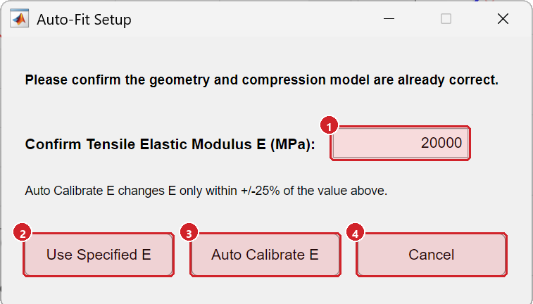
- Confirm the modulus. The box shows the tensile modulus from the Tension Model tab. Type a measured value here if you have one.
- Use Specified E keeps the modulus fixed and fits the cracking strain and the six post-cracking coordinates. Choose this when the modulus is known.
- Auto Calibrate E lets the modulus move within 25 percent of the value above while everything else is fitted. Choose this when the initial slope of the test does not match the simulation.
- Cancel returns without fitting.
The fit takes a few seconds for a typical file. When it finishes, the Tension Model boxes hold the fitted law and the simulated curve is drawn over the test. Press Update Results to refresh the other tabs. A fit is one undo step, so Ctrl+Z restores the previous law.
Judging the fit
The simulated curve should pass through the first-crack load, the peak and the tail. Compare the fitted \(E\) and \(\varepsilon_{cr}\) with the suggested values; a large difference usually means a wrong span, load spacing or unit. See Auto-Fit, the inverse analysis for the solver and its limits.
Step 6 · Read the results
Moment-Curvature
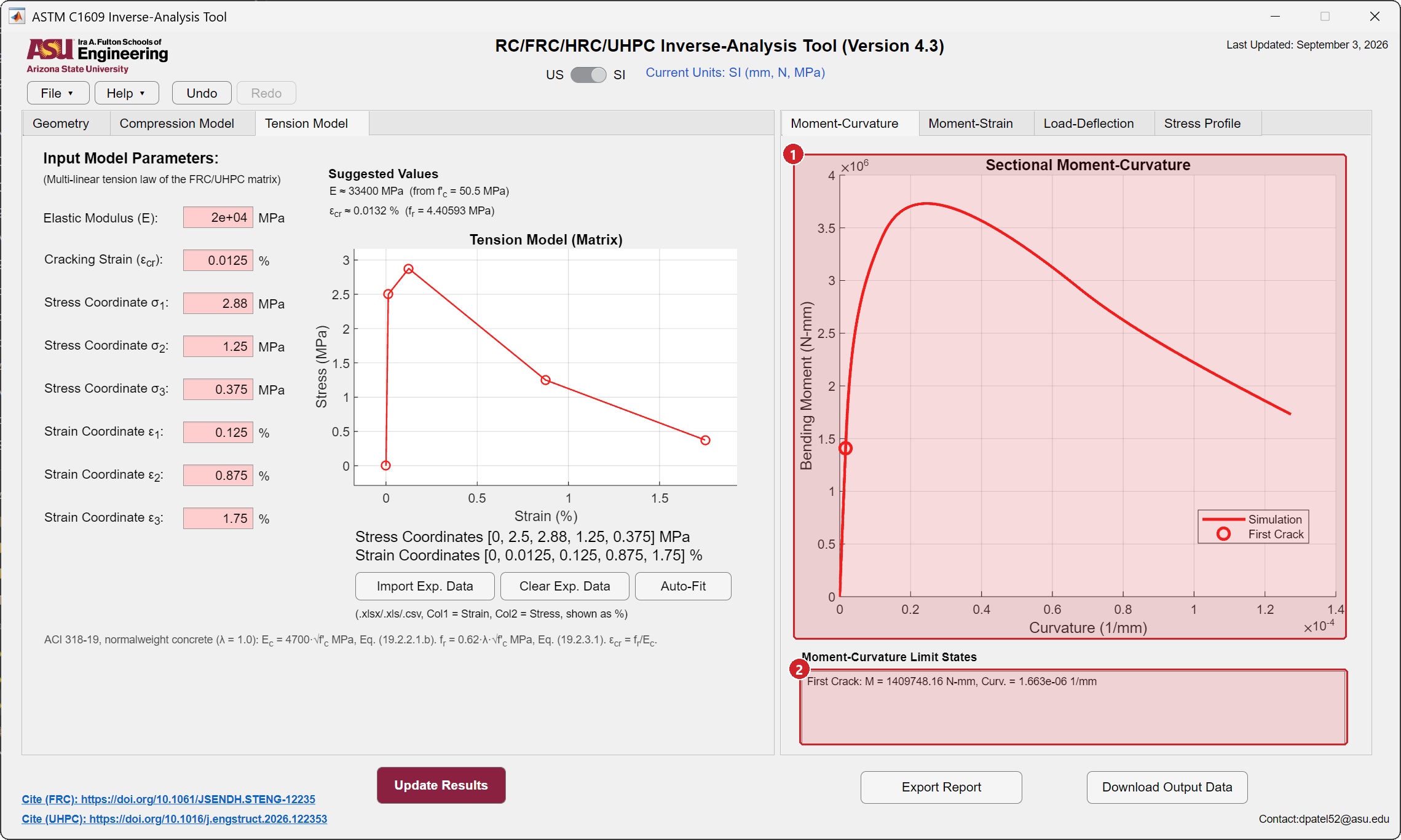
- The sectional moment-curvature curve computed from the fitted laws, with the limit states marked.
- Limit states. Moment and curvature at first crack and at compression yield when it is reached.
Moment-Strain
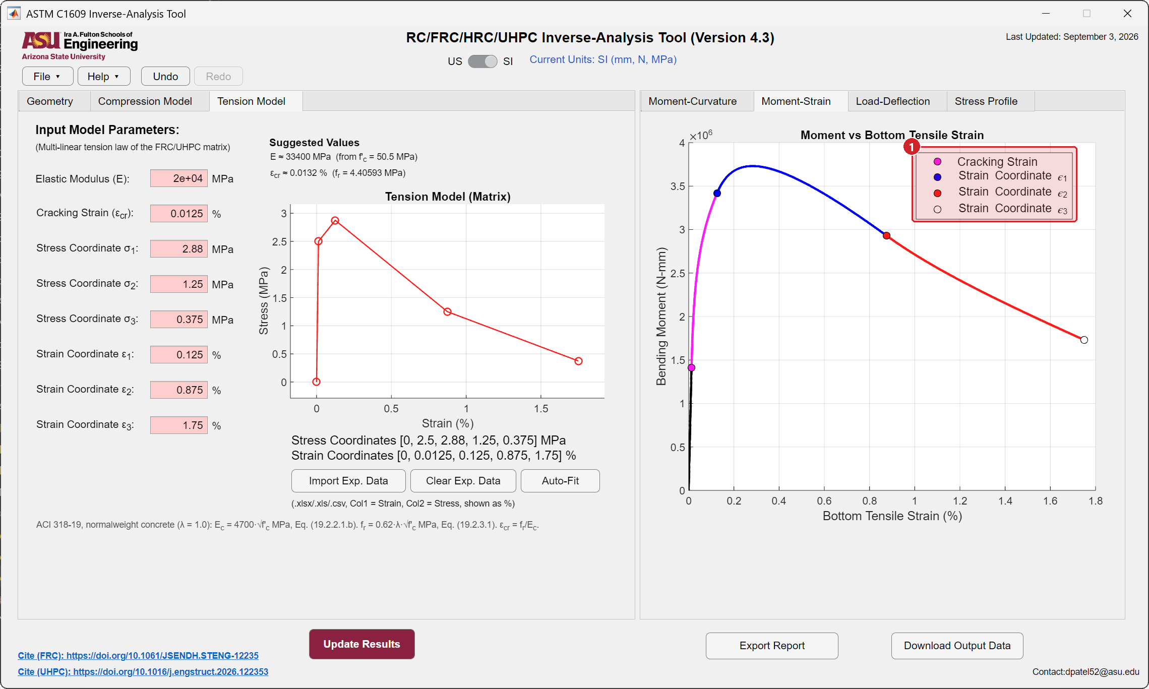
- Colors follow the tension law. Each segment of the curve is colored by the branch of the tension law that the bottom fiber is on, with markers at the cracking strain and at \(\varepsilon_1\), \(\varepsilon_2\) and \(\varepsilon_3\). It shows which coordinate controls which part of the response.
Stress Profile
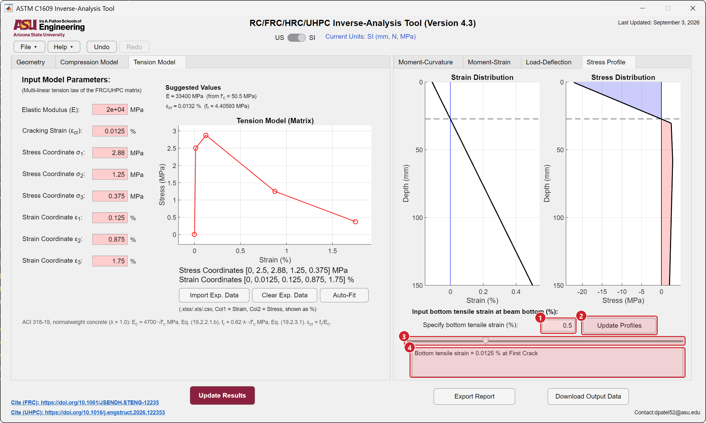
- Bottom tensile strain. Type the strain at which the profiles are drawn, in percent.
- Update Profiles redraws the strain and stress distributions through the depth. The dashed line is the neutral axis.
- Slider. Sweeps the strain from zero to \(\varepsilon_3\) and redraws continuously.
- State. Which limit state the chosen strain corresponds to.
Step 7 · Export and save
- Export Report writes the HTML report with the fitted law, the limit states and every figure.
- Download Output Data writes the workbook. Its
Input_Parameterssheet carries the fitted tension and compression laws into the Hybrid beam, FRP and Cross-sectional modules through File → Import Material. - File → Save keeps the whole session as a project file.
Worked example
Download ASTM_C1609_first_example_SI.mat and open it with File → Open. The beam is 150 × 150 mm on a 450 mm span in four-point bending with a load spacing of 150 mm and a plastic length of 150 mm, SI units. Its record has 92 measured points and a peak load of 51.3 kN. The tension law stored with it is \(E\) = 20 000 MPa, \(\varepsilon_{cr}\) = 0.0125 percent, stresses 2.88, 1.25 and 0.375 MPa at 0.125, 0.875 and 1.75 percent strain. The simulated curve follows the measured one through the peak and along the whole softening branch.
A step-by-step version of this run, from the module selector to the exported report, is on Run your first example.
To repeat the fit: type any rough tension law, press Auto-Fit on the Load-Deflection tab, choose Use Specified E, and compare the result with the stored values. Then change the plastic length to 75 mm, press Update Results, and watch the post-peak branch steepen: the plastic length controls how much of the beam softens.