Closed-form moment-curvature

Background · 2 of 5

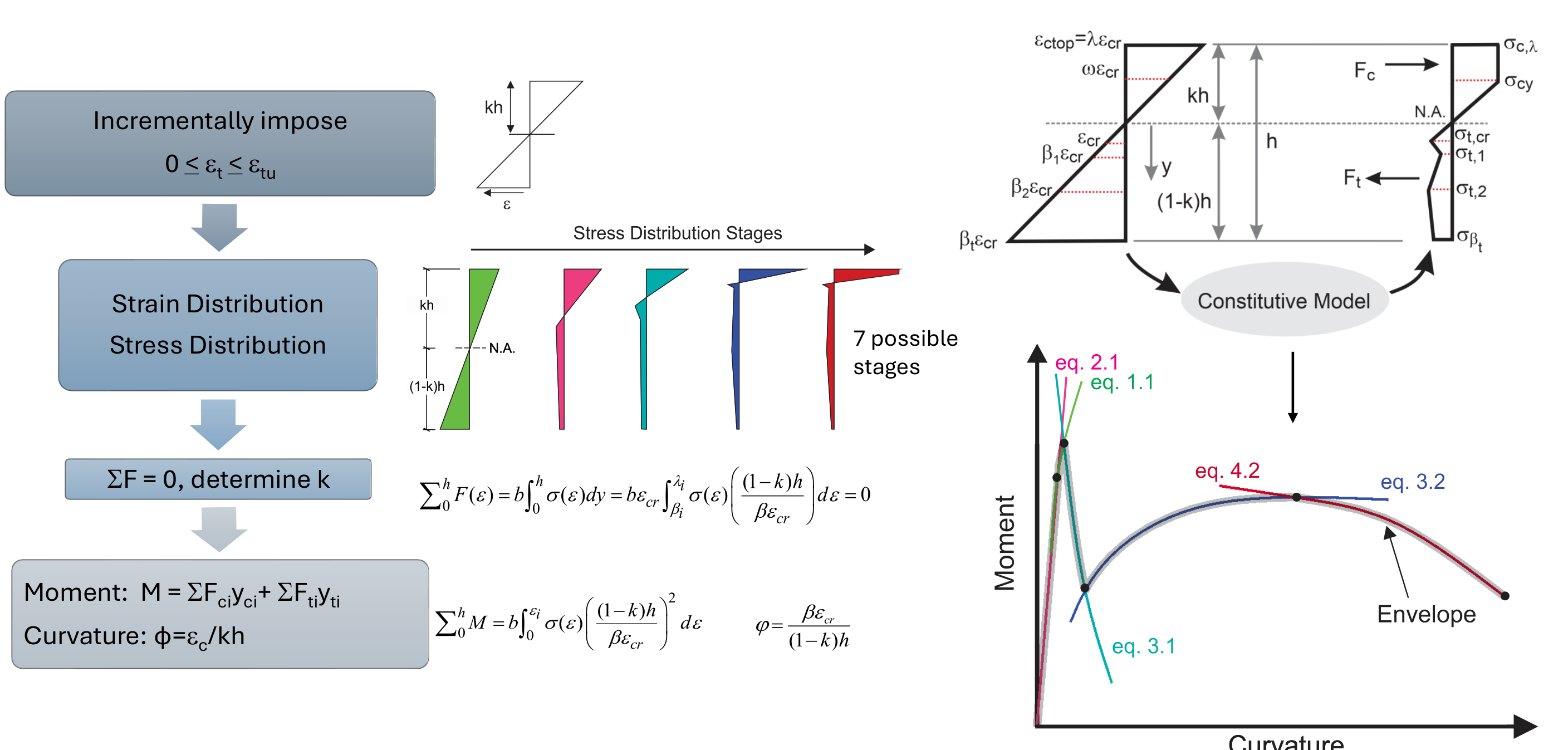
The section is solved by imposing the tensile strain at the bottom fiber and increasing it step by step. At every step the neutral axis follows from force equilibrium, and the moment and curvature follow from the neutral axis. Because every material law is piecewise linear, each step has a closed-form answer.

The moment-curvature model. Pleesudjai, C., Patel, D. D., and Mobasher, B. (2023). Generalized nonlinear moment-curvature model for serviceability-based design of hybrid reinforced concrete. Journal of Structural Engineering, 149(12), 04023188. doi:10.1061/JSENDH.STENG-12235

Formulation and limit states. Patel, D. D., Pleesudjai, C., Neithalath, N., and Mobasher, B. (2026). Limit-state based design of hybrid reinforced UHPC flexural beams using parametric modeling. Engineering Structures, 357, 122353. doi:10.1016/j.engstruct.2026.122353

One step of the solution. Impose the bottom strain, write the linear strain distribution, map it to stresses through the material laws, solve equilibrium for the neutral axis, integrate for the moment. Repeating the step traces the moment-curvature curve as an envelope of stages.

The three equations

With the bottom tensile strain \(\varepsilon_t = \beta\,\varepsilon_{cr}\) and the neutral axis at depth \(kh\), plane sections give the strain at any height \(y\) and the material laws give the stress. Equilibrium of the internal forces fixes \(k\):

\[ \sum F = b\int_0^{h} \sigma(\varepsilon(y))\,dy \;+\; \sum_j A_{s,j}\,\sigma_{s,j} \;=\; 0 \]

The moment is the first moment of the same stresses about the neutral axis, and the curvature is the strain gradient:

\[ M = b\int_0^{h} \sigma(\varepsilon(y))\,(y - kh)\,dy \;+\; \sum_j A_{s,j}\,\sigma_{s,j}\,(y_j - kh), \qquad \phi = \frac{\beta\,\varepsilon_{cr}}{(1-k)\,h} \]

For piecewise-linear laws every integral is a polynomial in \(k\), so the equilibrium equation is quadratic or lower and is solved without iteration. The software normalizes the moment by the cracking moment \(M_{cr} = \tfrac{1}{6} b h^2 \sigma_{cr}\) and the curvature by \(\phi_{cr} = 2\varepsilon_{cr}/h\).

Stages

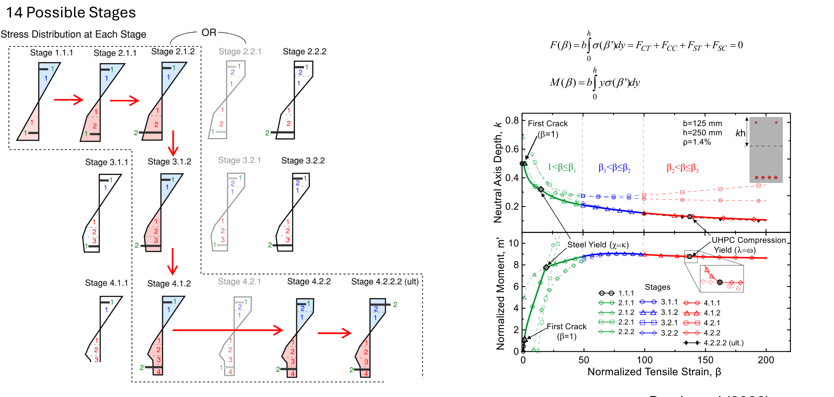
As \(\beta\) grows, the bottom fiber moves from the elastic branch into the post-cracking branches, the top fiber may reach compressive yield, and each rebar layer may yield. Every combination is a stage with its own closed-form pair \(k(\beta)\), \(M(\beta)\). The software evaluates all stages that are admissible at a given \(\beta\) and keeps the one that satisfies equilibrium, which produces the envelope shown in the figure above. A plain FRC section has 7 stages. A hybrid section with tension and compression rebar has up to 14. The stage boundaries are the limit states listed on the Moment-Curvature tab: first crack, compression yield, rebar yield, crushing and rupture.

Hybrid section. The stress distributions of the 14 possible stages of a beam with fibers and rebar, and the resulting neutral axis and moment curves against the normalized bottom strain.

What the tabs show

• Moment-Curvature. \(M\) against \(\phi\), with the limit states marked and listed.
• Moment-Strain. \(M\) against \(\beta\) or the bottom strain in percent, colored by the tension zone of the bottom fiber. It shows which coordinate of the tension law governs each part of the curve.
• Stress Profile. The strain and stress distributions through the depth at a chosen \(\beta\), with the neutral axis. The Force Profile tab of the design modules adds the resultant forces in the concrete and reinforcement.

Cross-sectional module

The Cross-Sectional Analysis module keeps the same material laws but replaces the closed form by a fiber discretization of an arbitrary polygon and solves equilibrium numerically at each curvature, with an axial load. This is what allows any shape, any number of rebar layers, prestressing tendons and the P-M interaction diagram. See Cross-sectional analysis.