Inverse analysis of EN 14651
Inverse analysis · notched beam · crack-width based
Back-calculate the tension stress-crack width law of an FRC from the load-CMOD curve of a notched prism in three-point bending, and read the EN 14651 residual strengths from the fitted response.
Upcoming EN 14651 workflow
This page describes the revised measured-CMOD workflow listed as Unreleased in the release notes. The available installer is version 4.3; its EN 14651 screens and results may differ. The 70A project and numerical results below belong to the revised workflow. For a first run, use the ASTM C1609 tutorial.
Method and validation. Patel, D., Pleesudjai, C., Bakhshi, M., Nasri, V., and Mobasher, B. (2025). Back-calculation of mechanical properties of fiber-reinforced concrete in tunnel lining segments. Structural Concrete, 26, 6019–6040. doi:10.1002/suco.70052
The software. Patel, D., Pleesudjai, C., and Mobasher, B. (2026). An interactive inverse-analysis and design tool for reinforced UHPC beams. Fourth International Interactive Symposium on Ultra-High Performance Concrete, paper 44.
Example data. Colombo, M., Conforti, A., di Prisco, M., Leporace-Guimil, B., Plizzari, G., and Zani, G. (2023). The basis for ductility evaluation in SFRC structures in MC2020: An investigation on slabs and shallow beams. Structural Concrete, 24, 4406–4423. doi:10.1002/suco.202300114
What you need
- The prism dimensions, the span and the notch depth. The EN 14651 prism is 150 × 150 mm, 500 mm span, 25 mm notch, loaded at midspan.
- The compressive strength of the mix.
- The load against CMOD record of one specimen as a two-column file, CMOD then load. The CMOD column is used exactly as measured; nothing is converted at import.
The 70A study, and the module's own example
This page uses the 70A study. The current local reference selection is a different SFRC prism, with 40 kg/m³ of fiber and a peak load of 15.1 kN, animated on the home page. Packaged examples may vary by build. To follow this study, download the 70A project above and open it with File → Open in a build using the revised measured-CMOD workflow.
Step 1 · Geometry
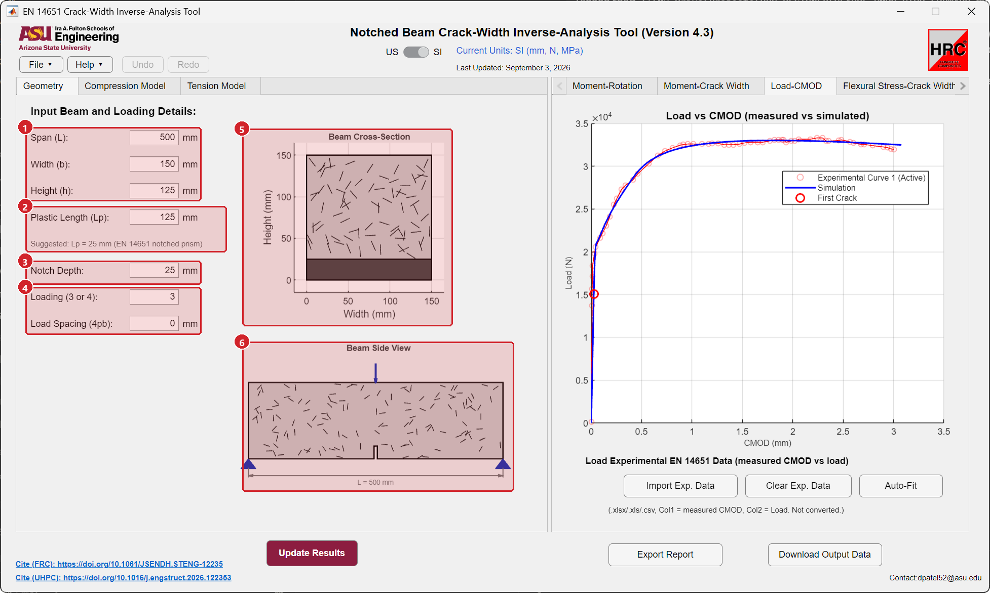
- Span, width and height. Height is the ligament depth above the notch, 125 mm for the standard prism. The notch is added below it in the drawings and in the flexural stress.
- Plastic length. The hinge length over which the crack opening is converted to rotation. The module suggests 25 mm. The example uses 125 mm, the ligament depth, which is the value its tension law was fitted with. The crack widths of the law and the plastic length belong together: change one and run Auto-Fit again.
- Notch depth. Depth of the sawn notch, 25 mm in the standard test.
- Loading and load spacing. 3 for the standard test. Enter 4 and a load spacing for a notched beam tested in four-point bending.
- Cross-section drawing. The notch is shown as the dark band at the bottom.
- Beam side view. Notch, support and load positions.
| Input | Symbol | Unit | Example |
|---|---|---|---|
| Span (L) | \(L\) | mm | 500 |
| Width (b) | \(b\) | mm | 150 |
| Height (h) | \(h\) | mm | 125 |
| Plastic Length (Lp) | \(L_p\) | mm | 125 |
| Notch Depth | \(d_n\) | mm | 25 |
| Loading (3 or 4) | 3 |
| Input | Symbol | Unit | Example |
|---|---|---|---|
| Span (L) | \(L\) | in | 19.7 |
| Width (b) | \(b\) | in | 5.91 |
| Height (h) | \(h\) | in | 4.92 |
| Plastic Length (Lp) | \(L_p\) | in | 4.92 |
| Notch Depth | \(d_n\) | in | 0.984 |
| Loading (3 or 4) | 3 |
Step 2 · Compression model
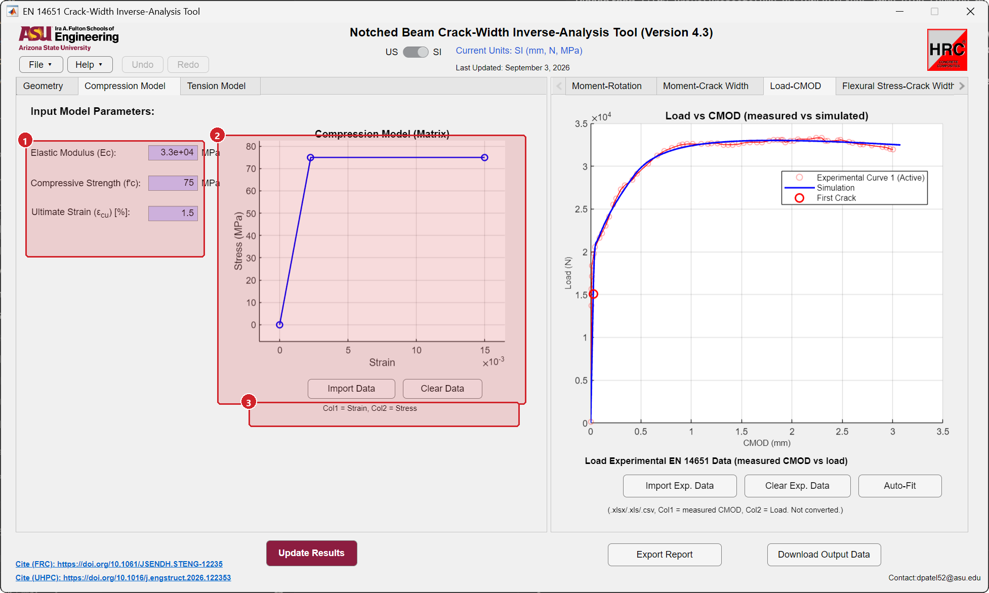
- Enter the compression law. Modulus \(E_c\), compressive strength \(f'_c\) and the ultimate strain \(\varepsilon_{cu}\) in percent. The law is elastic to the strength and then flat to the ultimate strain. The strength also sets the suggested tension values.
- Check the plot and drag a vertex if needed.
- Import and fit a measured compression curve, optional.
Step 3 · Tension model
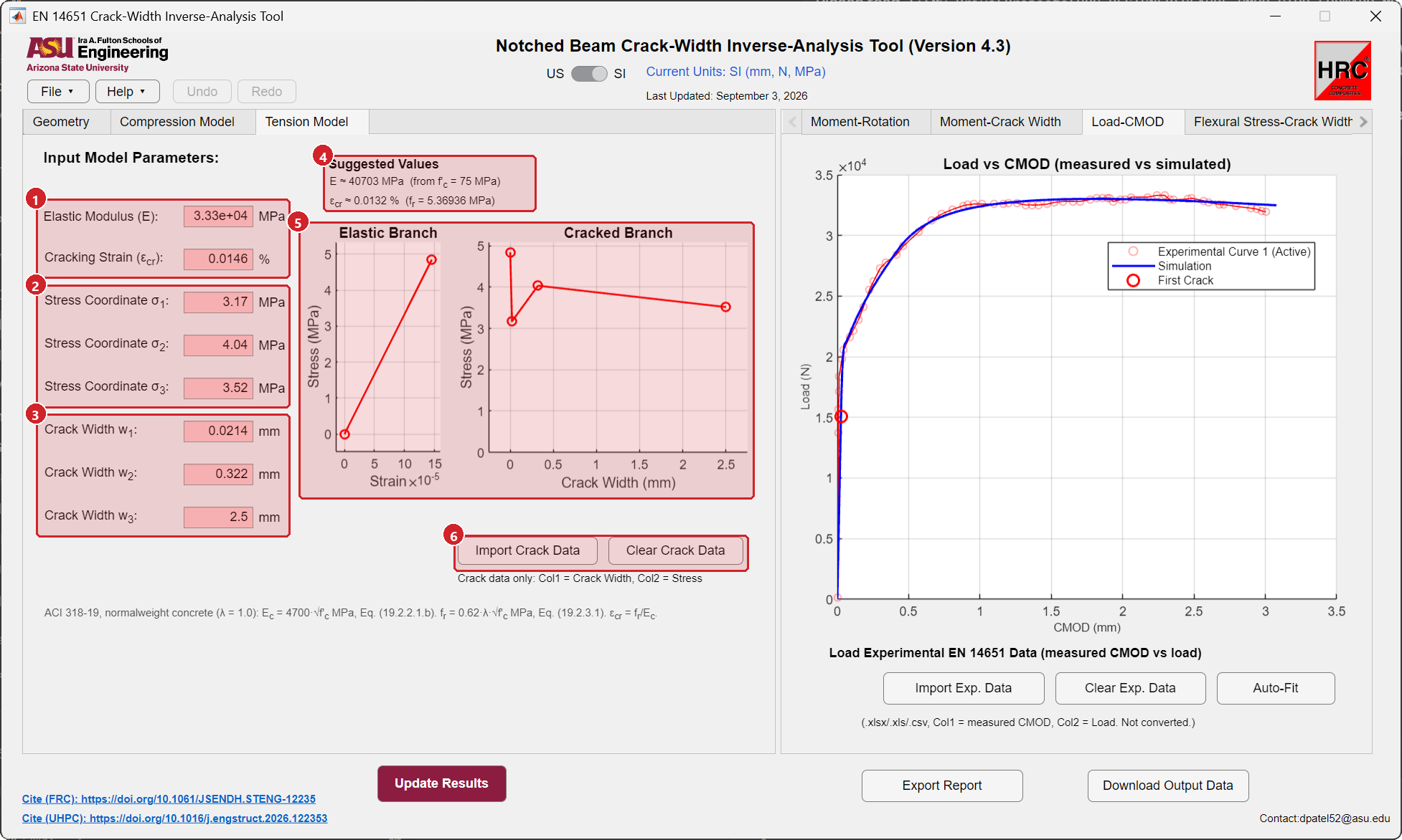
- Elastic branch. Modulus \(E\) and cracking strain \(\varepsilon_{cr}\). They fix the cracking stress \(\sigma_{cr} = E\,\varepsilon_{cr}\) and the response up to first crack.
- Stress coordinates. Three stresses \(\sigma_1, \sigma_2, \sigma_3\) carried across the crack.
- Crack widths. The crack openings \(w_1, w_2, w_3\) at which those stresses apply. They must increase. They live on the model's internal crack-opening coordinate, not on the measured CMOD, and Auto-Fit sizes \(w_3\) so that the simulated CMOD covers the whole measured record.
- Suggested values for \(E\) and \(\varepsilon_{cr}\) from the compressive strength.
- The two plots. Left, stress against strain up to cracking. Right, stress against crack width after cracking. Drag a vertex on either plot to change the law.
- Import Crack Data loads a measured stress-crack width curve, from a uniaxial tension test or a fiber pull-out model, to draw over the law.
| Input | Symbol | Unit | Example |
|---|---|---|---|
| Elastic Modulus (E) | \(E\) | MPa | 33 283 |
| Cracking Strain | \(\varepsilon_{cr}\) | % | 0.01456 |
| Stress Coordinate 1, 2, 3 | \(\sigma_1, \sigma_2, \sigma_3\) | MPa | 3.17, 4.04, 3.52 |
| Crack Width 1, 2, 3 | \(w_1, w_2, w_3\) | mm | 0.0214, 0.322, 2.50 |
| Input | Symbol | Unit | Example |
|---|---|---|---|
| Elastic Modulus (E) | \(E\) | psi | 4 827 000 |
| Cracking Strain | \(\varepsilon_{cr}\) | % | 0.01456 |
| Stress Coordinate 1, 2, 3 | \(\sigma_1, \sigma_2, \sigma_3\) | psi | 460, 585, 510 |
| Crack Width 1, 2, 3 | \(w_1, w_2, w_3\) | in | 0.00084, 0.0127, 0.0985 |
Step 4 · Import the test curve
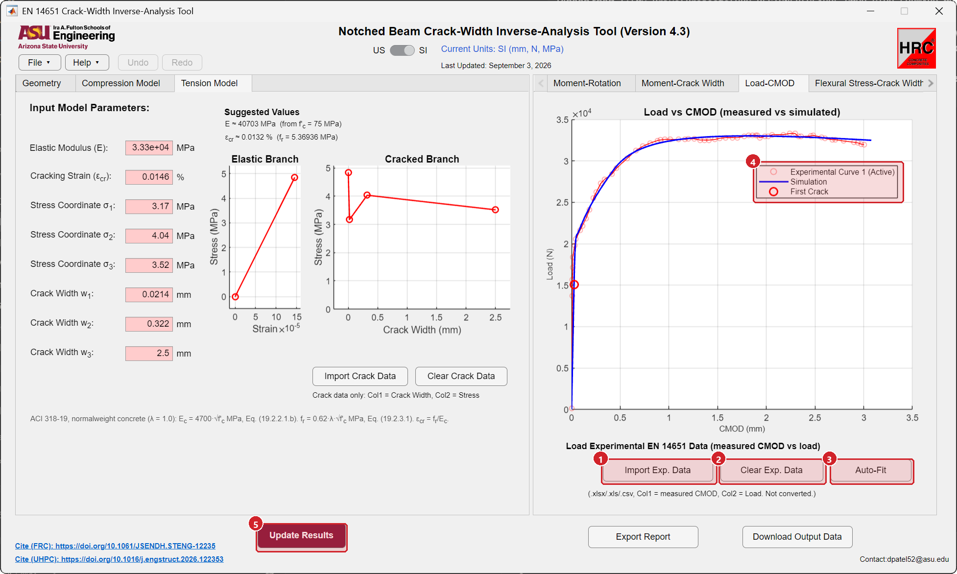
- Import Exp. Data. Choose the two-column file, measured CMOD then load. The CMOD column is stored and used exactly as read; there is no import conversion to choose.
- Clear Exp. Data removes the most recent curve.
- Auto-Fit starts the inverse analysis.
- Legend. Test curve, simulation, and the first-crack and compression-yield markers when they fall inside the response.
- Update Results recomputes after a manual change.
How the measured CMOD and the model CTOD are related
The clip gauge sits at the notch mouth, while the tension law is written on the opening at the notch tip. The module bridges the two in the forward direction: it never converts your data, it converts the model. For every trial law it builds the response, reads the neutral-axis ratio \(k\) and the total crack-tip opening
then transforms that forward to a simulated crack-mouth opening using the model's own kinematics,
with \(d_n\) the notch depth entered on the Geometry tab and \(h\) the remaining ligament. The simulated load is compared with the measured load at the measured CMOD positions. The experimental pairs never move, and no point is shifted or clamped.
The bracketed factor passes through the origin and falls as the crack grows. For the standard prism, \(h\) = 125 mm and \(d_n\) = 25 mm, it is 1.401 at first crack (\(k\) = 0.501 at \(\xi = E_c/E\) = 0.99) and tends to the geometric limit \((h+d_n)/h\) = 1.2 deep in the residual branch. A measured CMOD of 2.5 mm therefore corresponds to a model CTOD of roughly 2.05 mm on a standard specimen, which is why the crack widths \(w_1, w_2, w_3\) on the Tension Model tab are smaller than the CMOD values of the test.
Any CTOD reported against a measured CMOD station is a model-inferred CTOD, a property of the fitted law. A model-independent CTOD needs a direct measurement, such as digital image correlation or a gauge at the notch tip.
Removed in the upcoming release: the fixed CMOD-to-CTOD import conversion
Earlier builds offered a second import option that converts the measured CMOD through one fixed quadratic calibration, the same expression for every geometry and every material. Its positive intercept sends the smallest measured openings to negative crack widths, which then have to be clamped to zero, distorting the origin and the early slope from which \(E\) and \(\varepsilon_{cr}\) are identified. In the upcoming release it is removed and used nowhere in fitting, plotting or reporting. A project saved with that option warns when it is opened, because its stored x column is not measured CMOD; re-import the original record before trusting the fit, \(E\) or \(\varepsilon_{cr}\). The raw CMOD is deliberately not reconstructed by inverting the old polynomial.
Step 5 · Auto-Fit
Press Auto-Fit on the Load-CMOD tab. The Auto-Fit Setup dialog asks you to confirm the modulus and to choose Use Specified E or Auto Calibrate E. The solver then fits the cracking strain, the three stresses and the three crack widths to the active curve. A fit takes a few seconds on a 900-point file. Press Update Results afterwards to refresh every tab.
Step 6 · Read the results
Moment-Rotation and Moment-Crack Width
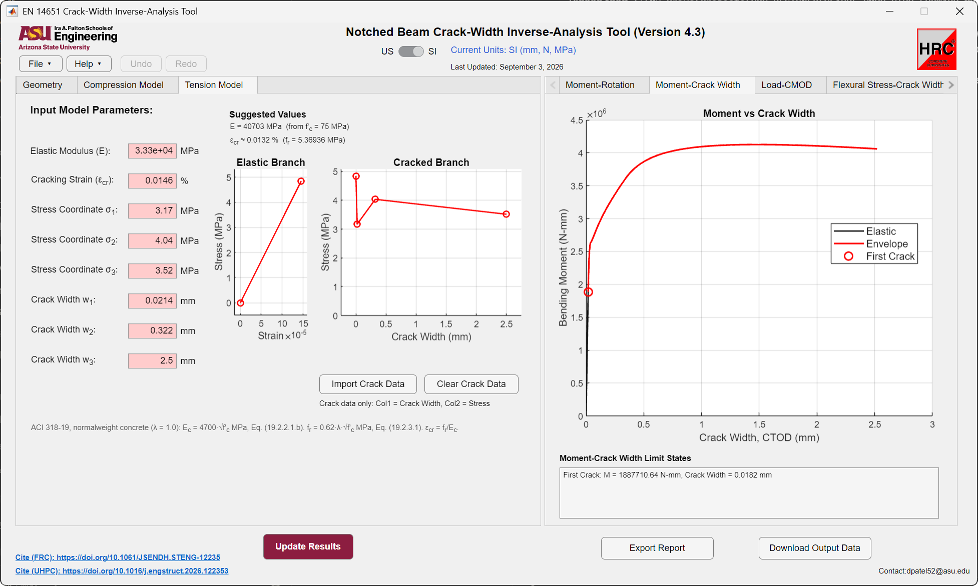
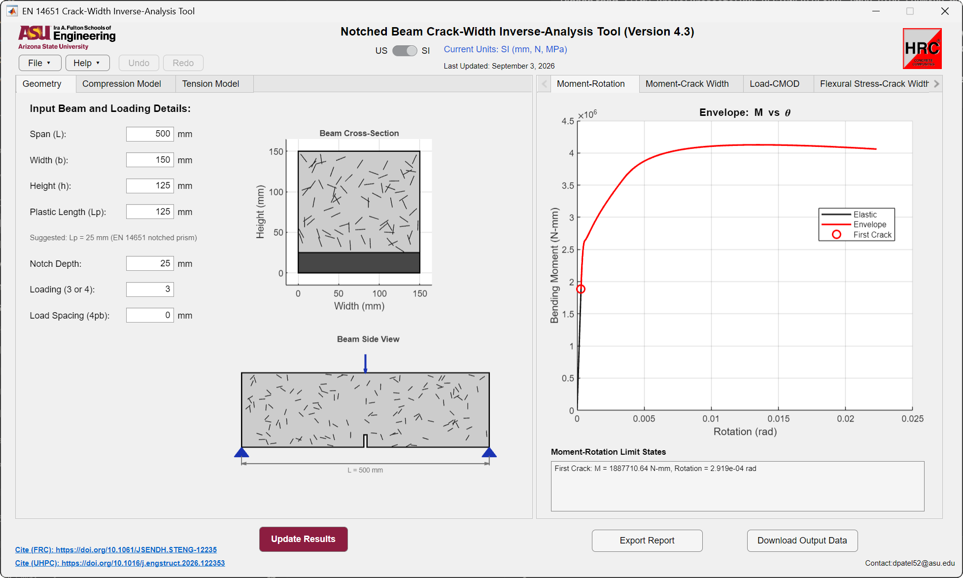
The section response of the notched hinge: the elastic branch, the envelope after cracking, the first-crack and compression-yield markers, and their values in the text box.
Flexural Stress-Crack Width
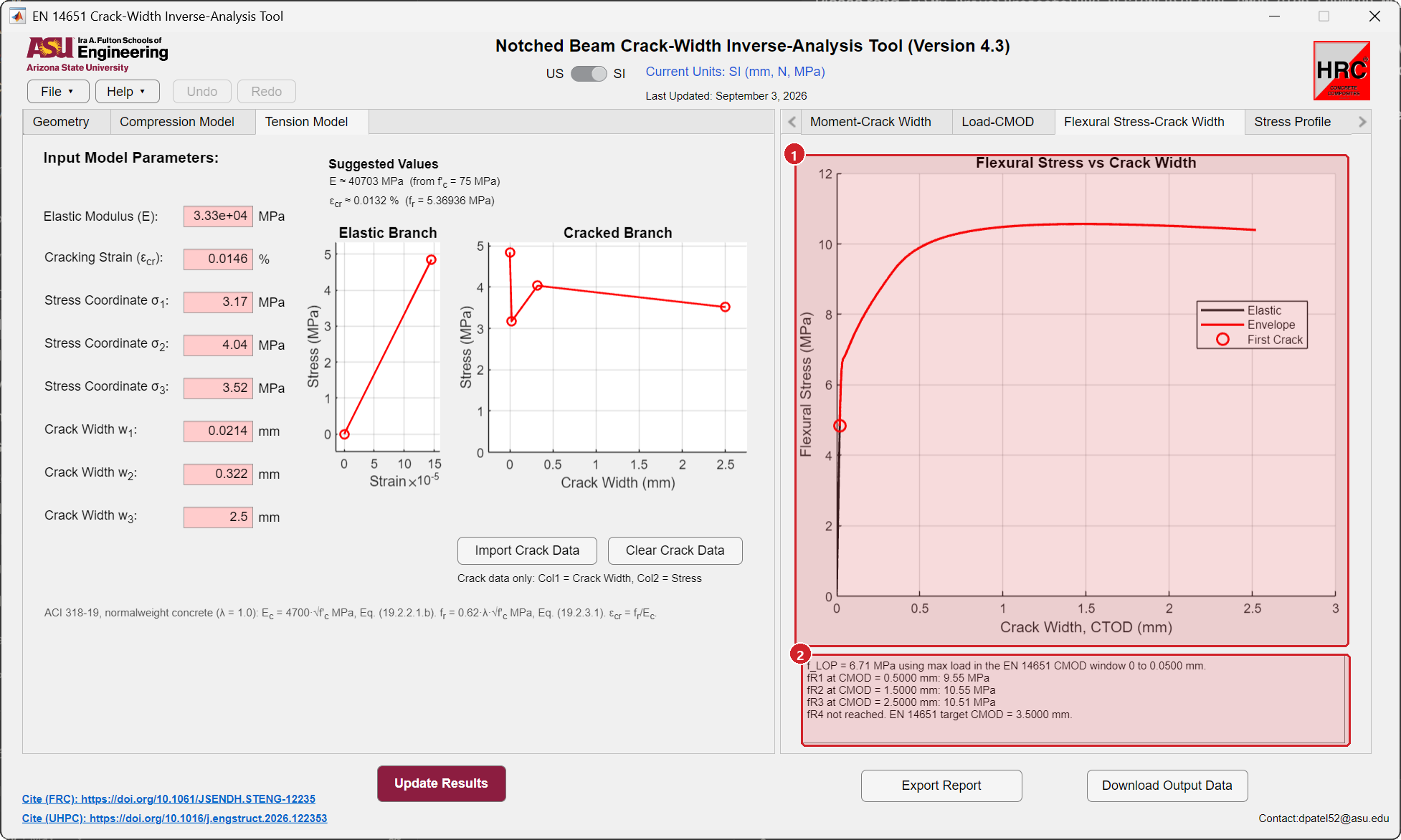
- Flexural stress \(f = 3FL/(2 b h_{sp}^2)\) against crack width, computed from the simulated load with the net ligament depth \(h_{sp} = h\), the Height entered on the Geometry tab. The notch is not subtracted again: the Height input is already the depth above the notch.
- Residual strengths. \(f_{LOP}\) from the largest load in the CMOD window 0 to 0.05 mm, and \(f_{R1}\) to \(f_{R4}\) at CMOD 0.5, 1.5, 2.5 and 3.5 mm, read from the fitted response. They are the values to enter in a fib Model Code or ACI 544 design.
Stress Profile
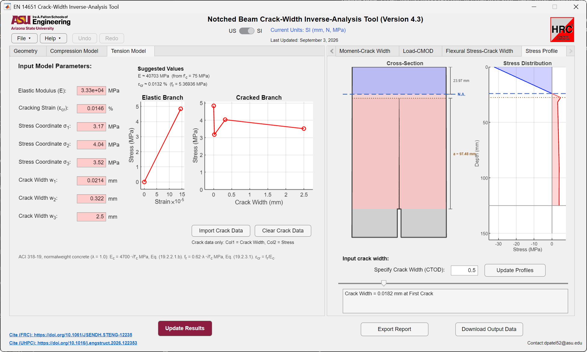
Type a crack width or move the slider, then Update Profiles. The strain distribution above the neutral axis and the stress distribution through the depth are drawn for that crack opening.
Step 7 · Export and save
Export Report, Download Output Data and File → Save work as in every module. The output workbook of this module carries a crack-width based tension law; the design modules convert it with the plastic length when it is imported.
Worked example
Download EN14651_70A_worked_example_SI.mat and open it with File → Open. The specimen is prism 70A of Colombo et al. (2023): 150 × 150 × 550 mm, 25 mm notch, 500 mm span, steel fiber type A (hooked-end, 60 mm long, 0.9 mm diameter) at 70 kg/m³, tested at the Politecnico di Milano. The record has 62 measured load-CMOD points to a CMOD of 3.00 mm and a peak load of 33.3 kN.
The law saved in this project, \(E\) = 33 283 MPa, \(\varepsilon_{cr}\) = 0.01456 percent, stresses 3.17, 4.04 and 3.52 MPa at internal crack openings 0.0214, 0.322 and 2.50 mm with \(L_p\) = 125 mm, was produced by Auto-Fit with Auto Calibrate E on the forward-CMOD workflow. Its simulated peak is 33.0 kN, 0.9 percent below the record, and its CMOD reaches 3.08 mm, just past the end of the test. Measured against the 62 recorded points the root-mean-square error is 7.6 percent of the peak load, but that number is carried almost entirely by the seven points inside the 0.05 mm limit-of-proportionality window, where the record rises almost vertically: from CMOD 0.05 to 0.5 mm the error is 1.1 percent of the peak, and beyond 0.5 mm it is 0.75 percent. The fit also reports that \(E\) landed on the edge of its search window, which is the honest signal that this record wants either a stiffer modulus or a longer \(L_p\).
The Flexural Stress-Crack Width tab reports \(f_{LOP}\) = 6.71 MPa and \(f_{R1}\), \(f_{R2}\), \(f_{R3}\) = 9.55, 10.55 and 10.51 MPa for this specimen; \(f_{R4}\) is not reported because the record stops at CMOD 3.00 mm, short of the 3.5 mm station. For the twelve prisms of the batch the paper reports averages of \(f_{ct,fl}\) = 6.50 MPa and \(f_{R1}\) to \(f_{R4}\) = 9.53, 10.49, 10.54 and 9.88 MPa, class 5d.
The model-inferred CTOD at the three reported stations is 0.399, 1.219 and 2.043 mm, against measured CMOD values of 0.5, 1.5 and 2.5 mm.
To repeat the fit, type a rough law on the Tension Model tab, press Auto-Fit on the Load-CMOD tab and compare. Then change the notch depth to 0 and press Update Results to see how much of the response the notch governs.
The law quoted above was fitted under the measured-CMOD workflow, which the release notes list under Unreleased. Builds using the earlier CMOD-to-crack-width conversion will not reproduce this fit because they optimise against the converted crack width.