Auto-Fit, the inverse analysis

Background · 4 of 5

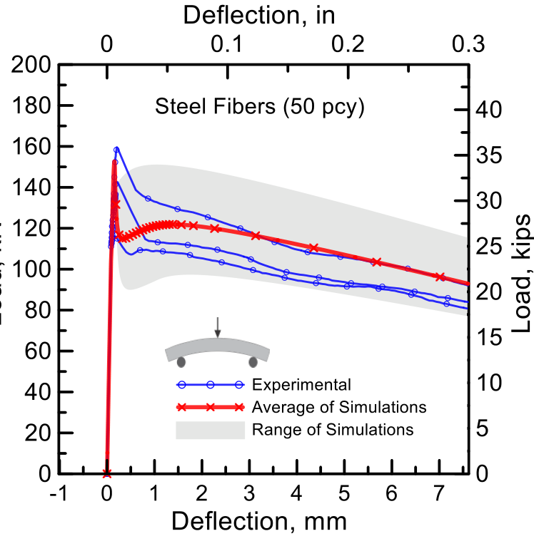
Inverse analysis means finding the tension law that reproduces a measured flexural curve. HRC Designer does this with a nonlinear least-squares solver wrapped around the closed-form forward model. Because one forward evaluation takes milliseconds, thousands of trials fit in seconds.

Method and validation. Patel, D., Pleesudjai, C., Bakhshi, M., Nasri, V., and Mobasher, B. (2025). Back-calculation of mechanical properties of fiber-reinforced concrete in tunnel lining segments. Structural Concrete, 26, 6019–6040. doi:10.1002/suco.70052

The software. Patel, D., Pleesudjai, C., and Mobasher, B. (2026). An interactive inverse-analysis and design tool for reinforced UHPC beams. Fourth International Interactive Symposium on Ultra-High Performance Concrete, paper 44.

The problem being solved

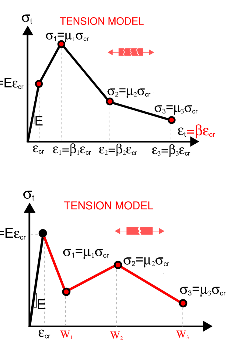
The unknowns are the post-cracking coordinates of the tension law and the cracking strain. The objective is the sum of squared differences between the measured load \(y_i\) and the simulated load \(\hat{y}_i\) at every recorded deflection, or in the notched-beam module at every recorded CMOD:

\[ S(\beta, \mu) = \sum_{i=1}^{n}\Big[\,y_i - \hat{y}_i(\beta, \mu)\,\Big]^2 \]

with \(\beta = (\varepsilon_{cr}, \beta_1, \beta_2, \beta_3)\) and \(\mu = (\mu_1, \mu_2, \mu_3)\) in the strain-based modules, and the crack widths \(w_1, w_2, w_3\) in place of the strains in the notched-beam module. The geometry and the compression law are held fixed. The tensile modulus \(E\) is either held at the value you confirm or allowed to move within 25 percent of it.

In the notched-beam module the \(x_i\) are the measured CMOD values and they never move. Each trial law builds its own response, and the crack-tip opening of that response is transformed forward to a simulated CMOD before the loads are compared, so the experimental record is never converted, shifted or clamped. The full relation is on the load-deflection page.

Version note. That forward-CMOD objective belongs to the EN 14651 change listed under Unreleased in the release notes. The solver, seeds and multistart procedure also apply to the earlier workflow.

Fitted laws. Strain-based (top) and crack-width based (bottom) tension laws. The red coordinates are the unknowns.

How the solver works

1. Seeds. A heuristic reads a starting guess off the experimental curve: the first-crack load gives the cracking strain, the peak and the tail give the post-cracking coordinates. The law currently typed in the Tension Model tab is a second seed. Both are tried.
2. Multistart. Several independent starts with randomized initial values run a coarse least-squares pass (MATLAB lsqnonlin, trust-region reflective, gradients by finite differences). This guards against the local minima of a seven-parameter problem.
3. Staged refinement. The best candidate is refined segment by segment, first the branch that controls the peak, then the softening tail, then all parameters together at tight tolerance.
4. Bounds. Every parameter stays inside physical bounds: increasing strain coordinates, positive stresses, a cracking strain within the range of concrete and UHPC.

The result is written into the Tension Model boxes and the simulated curve is drawn over the test. Press Update Results to refresh every other tab with the fitted law.

Judging a fit

• The simulated curve should follow the first-crack load, the peak load and the tail. A fit that matches the peak but misses the initial slope usually needs a different \(E\), so run again with Auto Calibrate E.
• A tail that crosses the data is a sign that the last strain coordinate is too small. Drag the last vertex on the Tension Model plot and watch the Load-Deflection tab update, then run Auto-Fit again from that seed.
• A fit that is good only near the peak can be improved by trimming the imported file to the range you trust. The solver weights every point equally.
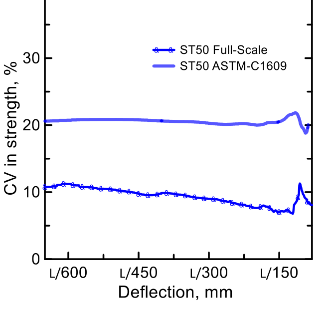
• Different specimens of the same mix should give laws that agree within the scatter of the test. Keep the fitted projects and compare them with the curve stack.

From one fit to a population

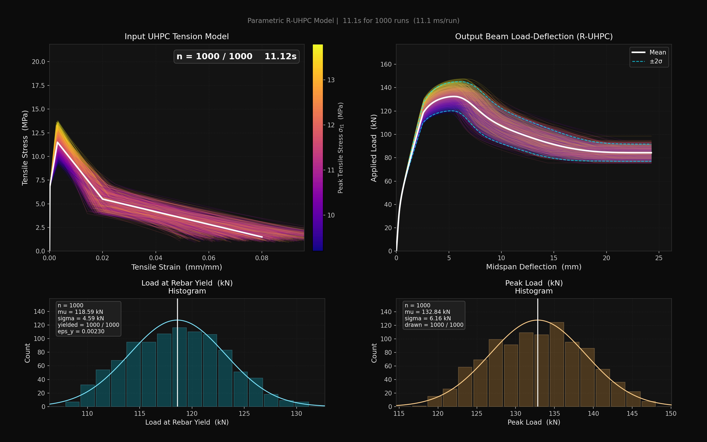
The same speed that makes Auto-Fit practical makes statistics practical. A fitted law is one sample of a material; the laws fitted to a batch of beams describe its scatter, and the forward model can be run over that scatter.

Scaling check. Tension laws back-calculated from ASTM C1609 beams (steel fibers, 50 pcy) were run on the full-scale tunnel segment. The average and the range of the simulations bracket the segment tests.

Variability scales with the section. The coefficient of variation in strength of the ASTM C1609 beams and of the full-scale segments, whose cross-section is ten times larger, against deflection. The larger section halves the scatter (Patel et al., 2023).

Monte Carlo simulation of a hybrid UHPC beam. Tension model parameters drawn from their measured distributions (top left), the resulting family of load-deflection curves (top right), and the distributions of the load at rebar yield and of the peak load (bottom). One thousand runs of the closed-form model take 11 seconds. Available as an open-source library.